B14 full

The Baldwin 2014 2-site exact solution relaxation dispersion model for SQ CPMG-type data. This model is labelled as B14 full in relax.

The advantage of this code will be that you'll always get the right answer provided you've got 2-site exchange, in-phase magnetisation and on-resonance pulses.

Equation

The paper main equation 50
[math] R_{2,\textrm{eff}} = \frac{R_2^A+R_2^B+k_{\textrm{EX}}}{2}-\frac{N_{\textrm{CYC}}}{T_{\textrm{rel}}}\cosh{}^{-1}(v_{1c}) - \frac{1}{T_{\textrm{rel}}}\ln{\left( \frac{1+y}{2} + \frac{1-y}{2\sqrt{v_{1c}^2-1}}(v_2 + 2k_{\textrm{AB}}p_D )\right)} \\ = R_{2,\textrm{eff}}^{\textrm{CR72}} - \frac{1}{T_{\textrm{rel}}}\ln{\left( \frac{1+y}{2} + \frac{1-y}{2\sqrt{v_{1c}^2-1}}(v_2 + 2k_{\textrm{AB}}p_D )\right)} [/math]

Which have these following definitions
[math] v_{1c} = F_0\cosh{\left(\tau_{\textrm{CP}}E_0\right)}-F_2\cosh{\left(\tau_{\textrm{CP}}E_2\right)} \\ v_{1s} = F_0\sinh{\left(\tau_{\textrm{CP}}E_0\right)}-F_2\sinh{\left(\tau_{\textrm{CP}}E_2\right)} \\ v_{2}N = v_{1s}\left(O_B-O_A\right)+4O_B F_1^a \sinh{\left(\tau_{\textrm{CP}}E_1\right)} \\ p_D N = v_{1s} + \left(F_1^a+F_1^b\right)\sinh{\left(\tau_{\textrm{CP}}E_1\right)}\\ v_3 = \left( v_2^2 + 4 k_{\textrm{BA}} k_{\textrm{AB}} p_D^2 \right)^{1/2} \\ y = \left( \frac{v_{1c}-v_3}{v_{1c}+v_3} \right)^{N_{\textrm{CYC}}} [/math]

Note, [math] E_2 [/math] is complex. If |x| denotes the complex modulus:
[math] \cosh{\left(\tau_{\textrm{CP}}E_2\right)} = \cos{\left(\tau_{\textrm{CP}}|E_2|\right)} \\ \sinh{\left(\tau_{\textrm{CP}}E_2\right)} = i \sin{\left(\tau_{\textrm{CP}}|E_2|\right)} [/math]

The term [math]p_D[/math] is based on product of the off diagonal elements in the CPMG propagator (Supplementary Section 3).

It is interesting to consider the region of validity of the Carver Richards result. The two results are equal when the correction is zero, which is true when
[math] \sqrt{v_{1c}^2-1} \approx v_2 + 2k_{\textrm{AB}}p_D [/math]
This occurs when [math]k_{\textrm{AB}}p_D[/math] tends to zero, and so [math]v_2=v_3[/math].
Setting [math]k_{\textrm{AB}}p_D[/math] to zero, amounts to neglecting magnetisation that starts on the ground state ensemble and end on the excited state ensemble and vice versa.
This will be a good approximation when [math]p_A \gg p_B[/math].
In practise, significant deviations from the Carver Richards equation can be incurred if [math]p_B \gt 1\%[/math].
Incorporation of the correction term into equation (50), results in an improved description of the CPMG experiment over the Carver Richards equation.

Equation compared to Carver Richards 72

Please see the relax summary of the model parameters here.

These definitions comes from the papers "Supplementary Section 4. Relation to Carver Richards equation".

[math] \tau_{\textrm{CP}} = \frac{1}{4\nu_\textrm{CPMG}} \\ \alpha_- = R_2^A - R_2^B + k_{\textrm{AB}} - k_{\textrm{BA}} \\ \zeta = 2 \Delta \omega \, \alpha_- = h_1\\ \Psi = \alpha_-^2 + 4 k_{\textrm{BA}} k_{\textrm{AB}} - \Delta \omega^2 = h_2\\ \xi = \frac{2\tau_{\textrm{CP}}}{\sqrt{2}}\sqrt{\Psi + \sqrt{\Psi^2 + \zeta^2}} = 2h_3 \tau_{\textrm{CP}} = \tau_{\textrm{CP}}E_0\\ \eta = \frac{2\tau_{\textrm{CP}}}{\sqrt{2}}\sqrt{-\Psi + \sqrt{\Psi^2 + \zeta^2}} = 2h_4 \tau_{\textrm{CP}} = \tau_{\textrm{CP}}E_2\\ D_+=\frac{1}{2}\left(1+\frac{\Psi+2\Delta \omega^2}{\sqrt{\Psi^2+\zeta^2}} \right) = F_0 \\ D_-=\frac{1}{2}\left(-1+\frac{\Psi+2\Delta \omega^2}{\sqrt{\Psi^2+\zeta^2}} \right) = F_2 [/math]

Physical meanings:
[math]\xi[/math] and [math]\eta[/math] are differences of the real and imaginary components of the free precession frequencies [math]f_{00}[/math] and [math]f_{11}[/math] (equation (41)).
[math]D_+[/math] and [math]D_-[/math] are the stay/stay ([math]F_{0}[/math]), and swap/swap ([math]F_{2}[/math]) coefficients (equation (36)).
[math]\zeta[/math] and [math]\Psi[/math] are parameters that enable the free precession frequencies to be written in a more concise form (equation (12)).
Note that in reference 2 (10.1016/S0076-6879(01)39315-1), in equation 25, the definition used for [math]\tau_{\textrm{CP}}[/math] is twice that used in this work but is otherwise identical.

Parameters

The B14 model has the parameters {$R_{2A}^0$, $R_{2B}^0$, $...$, $p_A$, $\Delta\omega$, $k_{ex}$}.

Code

Commits that created the code, approx 20-30 commits, with corrections.

Here is gna.org tracker that followed this code. It includes valuable comments.

The library code.
http://svn.gna.org/viewcvs/*checkout*/relax/trunk/lib/dispersion/b14.py?revision=HEAD

The target function. The func_B14_full().
http://svn.gna.org/viewcvs/*checkout*/relax/trunk/target_functions/relax_disp.py?revision=HEAD

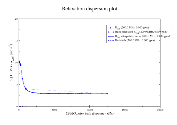
Example graph of test data

Graph from systemtest "relax -s Relax_disp.test_baldwin_synthetic"

Reference

The reference for the B14 model is:

• A.J. Baldwin (2014). An exact solution for R2,eff in CPMG experiments in the case of two site chemical exchange. J. Magn. Reson., 2014. (10.1016/j.jmr.2014.02.023).

Related models

The B14 model is a linear correction to the CR72 model, and algorithms based on this have significant advantages in both precision and speed over existing formulaic approaches.

Links

The implementation of the B14 full model in relax can be seen in the:

• relax manual,
• API documentation,
• relaxation dispersion page of the relax website.