Difference between revisions of "Tutorial for sorting data stored as numpy to on-resonance R1rho analysis"
| Line 50: | Line 50: | ||
| script = | | script = | ||
import os | import os | ||
| − | + | from scipy.io import loadmat | |
| − | |||
import numpy as np | import numpy as np | ||
# Set path | # Set path | ||
| + | #cwd = status.install_path+os.sep+'test_suite'+os.sep+'shared_data'+os.sep+'dispersion'+os.sep+'Paul_Schanda_2015_Nov' | ||
cwd = os.getcwd() | cwd = os.getcwd() | ||
| + | outdir = cwd + os.sep | ||
fields = [600, 950] | fields = [600, 950] | ||
| Line 70: | Line 71: | ||
# Loop over the experiments, collect all data | # Loop over the experiments, collect all data | ||
for field in fields: | for field in fields: | ||
| − | print(" | + | print("%s"%field,) |
# Make a dic inside | # Make a dic inside | ||
| Line 76: | Line 77: | ||
# Construct the path to the data | # Construct the path to the data | ||
| − | path = cwd + os.sep | + | path = cwd + os.sep |
| − | |||
# Collect all filename paths | # Collect all filename paths | ||
| Line 83: | Line 83: | ||
for file_name in file_names: | for file_name in file_names: | ||
# Create path name | # Create path name | ||
| − | file_name_path = path + "%s.mat"%file_name | + | file_name_path = path + "%s_%s.mat"%(field, file_name) |
field_file_name_paths.append(file_name_path) | field_file_name_paths.append(file_name_path) | ||
# Load the data | # Load the data | ||
| − | file_name_path_data = | + | file_name_path_data = loadmat(file_name_path) |
# Extract as numpy | # Extract as numpy | ||
file_name_path_data_np = file_name_path_data[file_name] | file_name_path_data_np = file_name_path_data[file_name] | ||
| Line 94: | Line 94: | ||
all_data['%s'%field]['np_%s'%file_name] = file_name_path_data_np | all_data['%s'%field]['np_%s'%file_name] = file_name_path_data_np | ||
| − | print | + | print(file_name, file_name_path_data_np.shape) |
# Collect residues | # Collect residues | ||
| Line 109: | Line 109: | ||
# Write a sequence file for relax | # Write a sequence file for relax | ||
| − | f = open("residues.txt", "w") | + | f = open(outdir + "residues.txt", "w") |
f.write("# Residue_i\n") | f.write("# Residue_i\n") | ||
for res in all_res_uniq: | for res in all_res_uniq: | ||
| Line 115: | Line 115: | ||
f.close() | f.close() | ||
| − | f_exp = open("exp_settings.txt", "w") | + | f_exp = open(outdir + "exp_settings.txt", "w") |
f_exp.write("# sfrq_MHz RFfield_kHz file_name\n") | f_exp.write("# sfrq_MHz RFfield_kHz file_name\n") | ||
# Then write the files for the rates | # Then write the files for the rates | ||
| + | k = 1 | ||
for field in all_data['fields']: | for field in all_data['fields']: | ||
resis = all_data['%s'%field]['np_residues'][0] | resis = all_data['%s'%field]['np_residues'][0] | ||
| Line 125: | Line 126: | ||
RFfields = all_data['%s'%field]['np_RFfields'][0] | RFfields = all_data['%s'%field]['np_RFfields'][0] | ||
| − | print("\nfield: %3.3f" % field) | + | print("\nfield: %3.3f"%field) |
for i, RF_field_strength_kHz in enumerate(RFfields): | for i, RF_field_strength_kHz in enumerate(RFfields): | ||
| − | #print | + | #print "RF_field_strength_kHz: %3.3f"%RF_field_strength_kHz |
# Generate file name | # Generate file name | ||
| − | f_name = "sfrq_%i_MHz_RFfield_%1. | + | f_name = outdir + "sfrq_%i_MHz_RFfield_%1.3f_kHz_%03d.in"%(field, RF_field_strength_kHz, k) |
cur_file = open(f_name, "w") | cur_file = open(f_name, "w") | ||
cur_file.write("# resi rate rate_err\n") | cur_file.write("# resi rate rate_err\n") | ||
| − | exp_string = "%11.7f %11.7f %s\n" % (field, RF_field_strength_kHz, f_name) | + | exp_string = "%11.7f %11.7f %s\n"%(field, RF_field_strength_kHz, f_name) |
| − | print(exp_string) | + | print("%s"%exp_string,) |
f_exp.write(exp_string) | f_exp.write(exp_string) | ||
| Line 144: | Line 145: | ||
cur_file.close() | cur_file.close() | ||
| + | k += 1 | ||
f_exp.close() | f_exp.close() | ||
Revision as of 15:32, 22 November 2015
Contents
Data background
This is data recorded at 600 and 950 MHz.
This should follow relax-4.0.0.Darwin.dmg installation on a Mac, only with GUI.
For each spectrometer frequency, the data is saved in np.arrays
- one for the residue number,
- one for the rates,
- one for the errorbars,
- one for the RF field strength.
They can be retrieved also with scipy's loadmat command.
The experiments are on-resonance R1ρ, and the rates are already corrected for the (small) offset effect, using the experimentally determined R1.
Specifically, the numpy shapes of the data is:
- For 600 MHz
- residues (1, 60)
- rates (60, 10)
- errorbars_rate (60, 10)
- RFfields (1, 10)
- For 950 Mhz
- residues (1, 61)
- rates (61, 19)
- errorbars_rate (61, 19)
- RFfields (1, 19)
For the 950 MHz, the 4000 Hz dispersion point is replicated.
An example of the data at the 2 fields is:
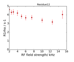
600 MHz
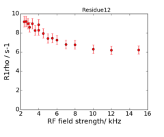
950 MHz


Create data files for relax
First prepare data, by running in Python:
python 1_prepare_data.py
The script is:
1_prepare_data.py script.Run analysis in relax GUI
- Start relax
- Then click: new analysis or ⌘ Cmd+n
- Then click icon for Relaxation dispersion → Next
- Just accept name for the pipe
- Open the interpreter: ⌘ Cmd+p
- Paste in
import os; os.chdir(os.getenv('HOME') + os.sep + 'Desktop' + os.sep + 'temp'); pwd()
- Then do
script(file='2_load_data.py')
- ( You can scroll through earlier commands with: ⌘ Cmd+↑ )
- Close the Grace
Results viewerwindow - Close the interpreter window
Now save the current state! This saved state can now be loaded just before an analysis, and contain all setup and data.
- File → Save as (Shift+Ctrl+S) → Save as
before_analysis.bz2
Now Quit relax, and start relax again.
Go to: File → Open relax state (Ctrl+O) → Locate before_analysis.bz2
In the GUI, select:
- For models, only select:
No RexandM61 - R1 parameter optimisation to False, as this on-resonance data does not use R1.
- The number of Monte-Carlo simulations to
3. (The minimum number before relax refuse to run). - Let other things be standard, and click execute
| Note The number of Monte-Carlo simulations is set to 3. This means that relax will do the analysis, and the fitted parameters will be correct, but the standard error of the parameters will be wrong. |
The reason for this is, that the data "naturally"? for some spins contains measurements which are "doubtful".
When relax is performing Monte-Carlo simulations, all the data is first copied x times to the number of Monte-Carlo simulations, and each R2,eff point on the graph
is modified randomly by a gaussian noise with a width described by the associated errors.
For spins which contains measurements which are "doubtful", relax will be spending "very long time" trying to fit a meaningful model.
This "time" is poorly spend on "bad data".
Rather, one should first try to
- analyse the data quickly
- make the graphs
- examine which spins should be deselected
- and then rerun the analysis with a higher number of monte-carlo simulations
After this comes the part with global fit/clustered analysis.
- analyse the data again
- Select which spins should be included in a global fit/clustered analysis
- and then rerun with analysis
The script
2_load_data.py script.Run the same analysis in relax through terminal
The analysis can be performed by
python 1_prepare_data.py

relax 2_load_data.py -t log.txt
# Or
mpirun -np 8 relax --multi='mpi4py' 2_load_data.py -t log.txt
Inspect and make graphs
- When this is done, quit relax
- Then to convert all xmgrace files to png
First make graphs
cd grace
./grace2images.py -t EPS,PNG

cd ..
cd No_Rex/
./grace2images.py -t EPS,PNG
cat r1rho_prime.out

cd ..
cd M61
./grace2images.py -t PNG
cat r1rho_prime.out
cat kex.out
cat phi_ex.out

cat kex.out | grep "None          12"
cat phi_ex.out | grep "None          12"
This should give the images of the data
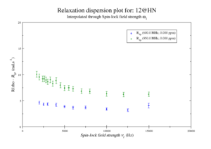
Resi 12 at 600+950 MHz

For model M61, spin 12 is:
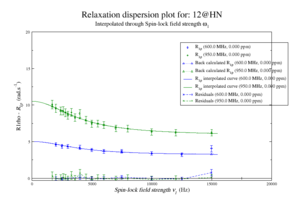
Resi 12 at 600+950 MHz for M61 model. kex=25000, phi_ex=0.32

Further analysis steps
- Inspect which residues should not be included in analysis
sel_ids = [
":4@HN",
":5@HN",
":6@HN",
":7@HN",
":10@HN",
":11@HN",
]
# De-select for analysis those spins who have bad data
deselect.all()
for sel_spin in sel_ids:
    print("Selecting spin %s"%desel_spin)
    select.spin(spin_id=desel_spin, change_all=False)
- Inspect which residues should be analysed together for a clustered/global fit.
cluster_ids = [
":13@N",
":15@N",
":16@N",
":25@N"]

# Cluster spins
for curspin in cluster_ids:
    print("Adding spin %s to cluster"%curspin)
    relax_disp.cluster('model_cluster', curspin)
- Run analysis again
See also
Bugs un-covered
- One data-point in spin 51, makes calculation go "nan", which makes relax go into infinity loop. This is an bug, and should be handled.
- The GUI is not updated when script 2 loaded, but only after spin deselection. There should be a "button" to force a "refresh" of the GUI.
- The "temp_state.bz" saved state can not be loaded in the GUI. Error message:
Traceback (most recent call last):
  File "gui/relax_gui.pyc", line 841, in state_load
  File "gui/relax_gui.pyc", line 893, in sync_ds
  File "gui/analyses/auto_relax_disp.pyc", line 646, in sync_ds
TypeError: int() argument must be a string or a number, not 'NoneType'
This probably due the above error
The spin 51 problem had nan in the original data.
import scipy.io
import numpy as np
a = "rates"
b = scipy.io.loadmat("/Users/tlinnet/Desktop/temp/Archive/exp_950/matrices/"+a+".mat")
c = b[a]
print np.isnan(np.min(c))

a = "errorbars_rate"
b = scipy.io.loadmat("/Users/tlinnet/Desktop/temp/Archive/exp_950/matrices/"+a+".mat")
c = b[a]
print np.isnan(np.min(c))