Difference between revisions of "Tutorial for sorting data stored as numpy to on-resonance R1rho analysis"
Jump to navigation
Jump to search
| Line 26: | Line 26: | ||
## RFfields (1, 19) | ## RFfields (1, 19) | ||
| − | + | <gallery heights=120px > | |
| − | |||
| − | |||
| − | |||
| − | |||
| − | <gallery heights= | ||
File:Residue12 600.png|600 MHz | File:Residue12 600.png|600 MHz | ||
File:Residue12 950.png|950 MHz | File:Residue12 950.png|950 MHz | ||
Revision as of 22:47, 14 November 2015
Data background
This is data recorded at 600 and 950 MHz.
For each spectrometer frequency, the data is saved in np.arrays
- one for the residue number,
- one for the rates,
- one for the errorbars,
- one for the RF field strength.
They can be retrieved also with scipy's loadmat command.
The experiments are on-resonance R1rho, and the rates are already corrected for the (small) offset effect, using the experimentally determined R1.
Specifically, the numpy shapes of the data is:
- For 600 MHz
- residues (1, 60)
- rates (60, 10)
- errorbars_rate (60, 10)
- RFfields (1, 10)
- For 950 Mhz
- residues (1, 61)
- rates (61, 19)
- errorbars_rate (61, 19)
- RFfields (1, 19)
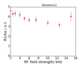
600 MHz
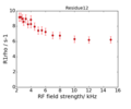
950 MHz


Create data files for relax
File: mat_example.py